The 2D Ising model implementation follows very closely the 1D model implementation. In particular define functions:
init(n).show(model).simulate(model, title, width, filename).energy(model).magnetization(model).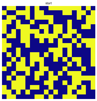
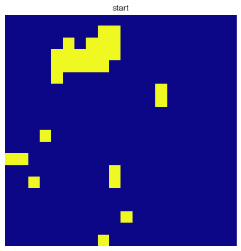
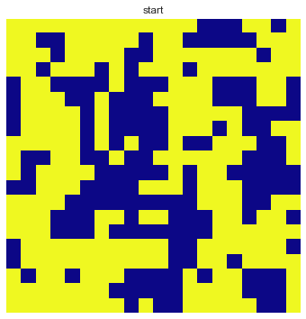
Example of the simulation output for low, middle, and high temperature are

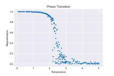
Taking random temperatures in range (0,5] we compute and store the final energy and magnetisation as in the 1D case. You should get graphs like the following:
Note: You can reduce simulation time by taking fewer Temperature points (here I'm taking 400), or be smarter about the values used. I used uniform random values over the range (0,5]. A good deterministic option is to use three different 'np.linspaceso you have more points over the interval of interest [1,3] and fewer points outside that. The output fromnp.linspaceis annp.arrayand multiplenp.arrays can concatenated usingnp.hstack`


Clearly something happens around 2 (actually around 2.26) can we estimate this point numerically? Yes, using curve fitting.
Looking at the absolute value of magnetisation against temperature we have

The curve appears to be
\[
f(T) = A \arctan\big[B\left(T-T_{critical}\right)\big] + C
\]
with parameters \(A\), \(B\), \(C\), and \(T_{critical}\).
However, before fitting it would be a good idea to remove all of the noise in the bottom left quarter of the figure. A np.where call will create a logical filter to do this for you. So you should perform the fit on the filtered data subset.
Now applying a curve fit (I used scipy.optimize.curve+fit, but you have many alternatives here) and plotting the fit with the original data I get
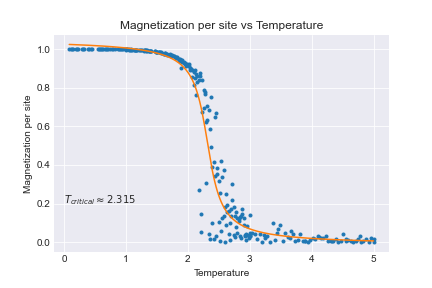
So my estimate of the critical temperature is 2.35.