Simulate the 2D Ising model and estimate the critical time at which phase transition occurs.
The Ising model is a very simple system that exhibits many of the characteristics of physical systems of large numbers of particles. In this lesson we will use the Ising model to investigate a phase transition between randomly ordered domains and uniformly aligned domains, representing the transition into ferromagnetism.
You are probably aware of the magnetisation properties of iron, and in particular the phase transition that occurs at 1000 K. Above this temperature, iron is no longer ferromagnetic. Instead, the individual domains of aligned atoms within the iron become randomly oriented. While the ferromagnetic and non-ferromagnetic behaviours are fundamentally different, both behaviours and the transition between can be modelled using the Ising model. The Ising model was first used in the 1920s to study this phase transition in ferromagnetism.
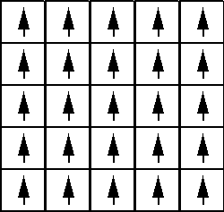
The n-D Ising model consists of an n-dimensional lattice of spins, which, in our application can either be up or down.


Imagine each of these spins was a tiny bar magnet, and all the magnets were aligned. If you tried to flip one of the magnets, you would have to do work on the system because you are fighting against the magnetic field of the neighbouring magnets; the magnets prefer to be aligned. We can model this effect by assuming that individual spins interact with their nearest neighbours, resulting in an interaction energy than depends on the relative alignment of the spins. If the individual spins can take on values of +1 or -1 (corresponding to up or down), we can write the total energy of the system as:
\[ E = -J \sum_{\begin{array}{c}\text{all cells}\\\text{\(i\)}\end{array}} \sum_{\begin{array}{c}\text{neighbours}\\ \text{of cell \(i\)}\end{array}} s_i s_j \]
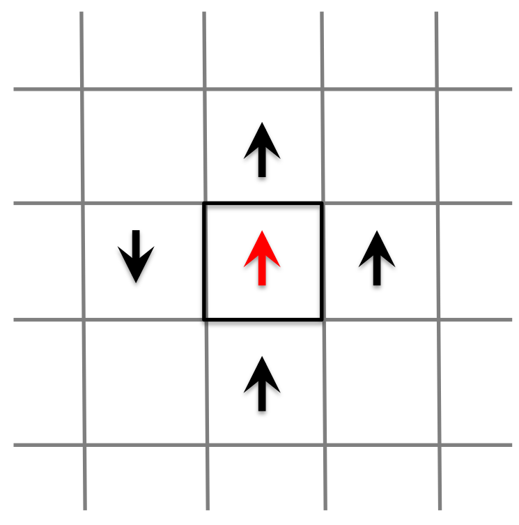
where the summation is over all (2 for 1D, 4 for 2D, 6 for 3D) the pairs of nearest neighbours in the system, and the 1/2 factor is to deal with counting spins twice. The parameter \(J\) is known as the exchange energy, and if this constant is positive, the spins prefer to be aligned. If you try to flip one spin in the system, you can use this equation to calculate the change in the energy of the entire system due to that spin flip. For instance, consider a random box in our lattice of spins, along with its four nearest neighbours:

Flipping the spin in this box would change the total energy of the whole system through the contribution of the interaction energy with its four nearest neighbours. Before flipping, this contribution is
\[ E_{before} = -J \frac{1}{2} \cdot (+1) \cdot ( -1 -1 -1 +1) = +2J \]
corresponding to 3 neighbours aligned with the spin in the centre cell (hence lower - negative - energy) and one spin aligned in the opposite direction (a high potential energy). After flipping, the contribution to the total energy of this cell would be
\[ E_{after} = -J \cdot (-1) \cdot ( - 1 - 1 - 1 + 1) = -2J \]
The change in the total energy of the system after flipping this one cell would be
\[ E_{\text{flip}} = E_{\text{after}} - E_{\text{before}} = -4J \]
So, if \(J\) is positive, this would decrease the energy of the system and hence it would be an energetically favourable change.
If this was all that was involved — driving the system to the lowest energy state — the end result would simply be all the cells aligned with each other. If \(E_{\text{flip}} > 0\) the process would require an input of energy into the system; this is where the concept of energy comes in. The basic idea is that the thermal energy of the system provides the means for flipping spins when \(E_{\text{flip}} > 0\). If the temperature is high (\(k_{B}T\) is high relative to \(E_{\text{flip}}\)), it will be easy to make energetically unfavourable flips because there is plenty of thermal energy available. Conversely, if the temperature is low, spins are not likely to flip when \(E_{\text{flip}} > 0\). Here \(k_B\) is Boltzmann's constant.
To implement this concept of thermal spin flips, we need to know the probability that a given (unfavourable) spin flip will occur as a function of temperature. We begin with the fundamental result of statistical mechanics that for a system in equilibrium with a heat bath at temperature \(T\), the probability of finding the system in any particular state \(m\) of energy \(E_m\) is proportional to the Boltzmann factor
\[ p = e^{ - E_m/ (k_{B} T) } \]
Hence, the probability of a system transitioning from a lower energy state (2) to a higher energy state (1) is given by
\[ P = e^{-(E_1 - E_2)/ (k_B T)} \]
Before we outline the simulation algorithm we need to focus on the issue of boundary cell behaviour. For example in the 2D model corner cells have only two neighbours, while other edge cells have three neighbours. Here we have a few options:
The algorithm for our Ising model should look something like this:
To help you implement this simulation I have broken it into separate tasks with expected output.
Create a colab notebook implementing the above tasks, reproducing the stated output. Download notebook and upload to Moodle using the following link