We will cover this task during the lab session, and will use a similar implementation for the main problem, the 2D Ising model.
To keep things simple we pick units so that both \(J\) and \(k_B\) are effectively one. Then the average energy per spin site is \[ \langle E\rangle = - \frac{1}{\text{number of sites}} \frac{1}{2} \sum_{ \begin{array}{c} \text{over all}\\ \text{sites \(i\)} \end{array} } \sum_{ \begin{array}{c} \text{over all}\\ \text{neighbours \(j\)} \end{array} } s_i \cdot s_j \] and the magnetisation per site is \[ \langle M\rangle = \frac{1}{\text{number of sites}} \sum_{ \begin{array}{c} \text{over all}\\ \text{sites \(i\)} \end{array} } s_i \] And the transition probability when flipping to a higher energy state (difference \(\Delta E\)) is \[ p = e^{-\Delta E / T} \]
Implement function
1 2 | |
which returns an 1D array of n elements. The each element are -1/+1 with probability 0.5. So a possible output of init(20) is
1 | |
Implement function
1 2 | |
which displays the model using plt.imshow using optional width and title. So a possible output of show(model, title="time = start") is

Implement function
1 2 | |
which computes the energy per spin site in model due to spin of neighbouring sites. This function should return values in range -1 (for all spin up) to 1 (all spin down).
Implement function
1 2 | |
which computes the bulk magnetisation per spin site in model. This function should return values in range -1 (for all spin down) to 1 (all spin up). (Note the difference with energy.)
Implement function
1 2 3 | |
which performs t_steps Monte Carlo iterations on model. I used the optional parameter debug to print out the usual debug info.
We can now use this function to study the behaviour of the model.
Using code like
1 2 3 4 5 6 7 8 | |
we are able to run a simulation of the same starting state under different conditions.
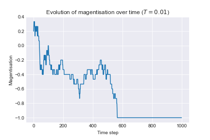
First when the temperature is low the transition probability limit for a site to flip to a higher state is closer to one so less likely to occur. Hence we expect a trend towards lower energy states
Taking the same initial state:

And re-running simulation for 10,000 steps with \(T=0.1\) we get


So system converges to either state where the spins are aligned.
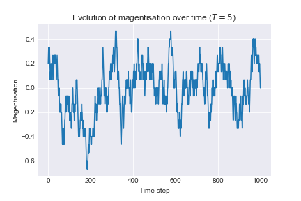
Re-running same experiment, using same initial state, for high temperature (\(T=5\)) get


So system don't get alignment of spins and at a local level, the prediction of spins is impossible.
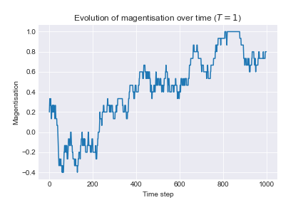
So what about temperatues that are not too low nor too high?
Re-running same experiment, using same initial state, for temperature (\(T=1\)) get


We get regions of spin alignment. I think the probability distribution of the size of regions is known but I know that I don't know it. These regions are not fixed and "slowly" change over time.
Rather than looking at the start and end point we can call the function simulate inside a for loop and compute the magnetisation over time, using code like:
1 2 3 4 5 6 7 | |
To examine the effect of temperature we run the following algorithm:
The corresponding code is
1 2 3 4 5 6 7 8 9 10 11 12 | |
and the resulting plot using
1 2 3 4 5 6 | |
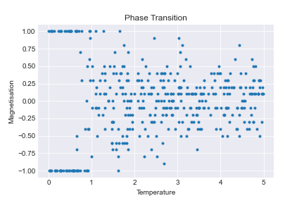
This is very noisy and difficult to see, so we need to tweak our algorithm by:
The updated code is
1 2 3 4 5 6 7 8 9 10 11 12 13 14 15 16 | |
and the resulting plot is
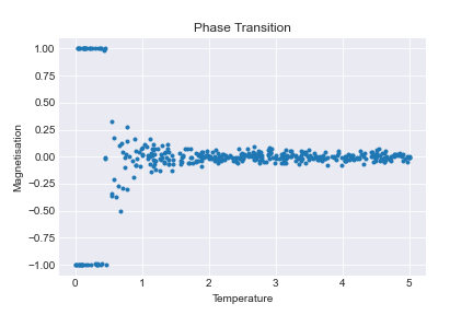
This is much better. Now we can see that something fundmental happens around \(T=1\), where the model switches from the low temperature state to the high temperature states. This temperature, \(T=1\), is called the critical temperature. We want to determine the corresponding critical temperature for the 2D model.
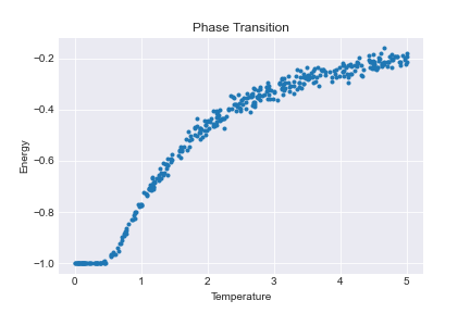
The corresponding energy plot is
There are a number of (optional) improvements that can be made to this implementation. In particular
simulate, and not parallelising the flipping of spins. Parallelising the flipping of spins by replacing the element operations in simulate array would result in a huge speedup but would break the Monte Carlo assumption of individual spins occurring and can lead to cyclic effects. There is a fix for this but that is for another day.